The plot_rates() plots prevalence/incidence rates
Usage
plot_rates(
  data,
  date_col = "date",
  rate_col,
  grouping_var = NULL,
  facet_var = NULL,
  plot_type = c("line", "bar_chart", "lollipop", "jitter"),
  percent = TRUE,
  palette = c("fhi_colors", "viridis", "okabe_ito"),
  single_color = "black",
  annotated_line = NULL,
  CI_lower = NULL,
  CI_upper = NULL,
  plot_title = "",
  x_name = "",
  y_name = "",
  legend_title = "",
  coord_flip = FALSE,
  start_end_points = FALSE,
  interactive = FALSE
)
Arguments
- data
A data frame with the prevalence/incidence rates and auxiliary information.
- date_col
A character string. Name of the date column in
data. Default is "date".- rate_col
A character string. Name of the rate column in
data.- grouping_var
A character string. Name of the variable/column in
dataused to group rates.- facet_var
A character string. Name of the variable/column in
dataused to facet plots.- plot_type
A character string. Type of plot, options are "line", "bar_chart", "lollipop", "jitter"
- percent
Logical. Do you want axis to be in percent? Default set to TRUE.
- palette
A character string. Color palette to be used in the plots, options are: "fhi_colors", "viridis", "okabe_ito"
- single_color
A character string. Single color applied to all the plot. Default is set to "black"
- annotated_line
Character string. Position of annotated line. Default is NULL.
- CI_lower
A character string. Name of the column containing the lower confidence interval in
data.- CI_upper
A character string. Name of the column containing the upper confidence interval in
data.- plot_title
Character string. Title of the plot.
- x_name
A character string. Title of the x axis.
- y_name
A character string. Title of the y axis.
- legend_title
A character string. Title for the legend box.
- coord_flip
Logical. Default is set to
FALSEFor lollipop, bar charts and jitter
TRUEit flips the orientation of the plot.
- start_end_points
Logical. Want to annotate the start and end points of a line plot? Default is set to
FALSE.If
TRUE, the start and end point of a line plot are annotated with their corresponding numerical values.
- interactive
Logical. Do you want to make the plot interactive with plotly? Default is set to FALSE.
Examples
log_file <- tempfile()
cat("Example log file", file = log_file)
pop_df <- tidyr::expand_grid(year = 2012:2020,
sex = as.factor(c(0, 1)),
innvandringsgrunn = c("ARB", "UKJ", "NRD")) |>
dplyr::mutate(population = floor(runif(dplyr::n(), min = 3000, max = 4000)))
linked_df <- linked_df |> dplyr::rename("year"= "y_diagnosis_first")
prev_series <- regtools::calculate_prevalence_series(linked_df,
time_points = c(2012:2020),
id_col = "id",
date_col = "year",
pop_data = pop_df,
pop_col = "population",
grouping_vars = c("sex", "innvandringsgrunn"),
only_counts = FALSE,
suppression = FALSE,
CI = TRUE,
CI_level = 0.95,
log_path = log_file)
#> Computing prevalence rates/counts...
#> ! No suppression. Confidentiality cannot be assured.
#> Joining with `by = join_by(sex, innvandringsgrunn, year)`
#>
#> ✔ Prevalence rates ready!
#>
#> ── Summary ─────────────────────────────────────────────────────────────────────
#> ℹ Diagnostic and demographic data: linked_data
#> ℹ Population data: pop_data
#> ℹ Grouped by variables: sex and innvandringsgrunn
#> ℹ For time point/period: 2012
#> Computing prevalence rates/counts...
#> ! No suppression. Confidentiality cannot be assured.
#> Joining with `by = join_by(sex, innvandringsgrunn, year)`
#>
#> ✔ Prevalence rates ready!
#>
#> ── Summary ─────────────────────────────────────────────────────────────────────
#> ℹ Diagnostic and demographic data: linked_data
#> ℹ Population data: pop_data
#> ℹ Grouped by variables: sex and innvandringsgrunn
#> ℹ For time point/period: 2013
#> Computing prevalence rates/counts...
#> ! No suppression. Confidentiality cannot be assured.
#> Joining with `by = join_by(sex, innvandringsgrunn, year)`
#>
#> ✔ Prevalence rates ready!
#>
#> ── Summary ─────────────────────────────────────────────────────────────────────
#> ℹ Diagnostic and demographic data: linked_data
#> ℹ Population data: pop_data
#> ℹ Grouped by variables: sex and innvandringsgrunn
#> ℹ For time point/period: 2014
#> Computing prevalence rates/counts...
#> ! No suppression. Confidentiality cannot be assured.
#> Joining with `by = join_by(sex, innvandringsgrunn, year)`
#>
#> ✔ Prevalence rates ready!
#>
#> ── Summary ─────────────────────────────────────────────────────────────────────
#> ℹ Diagnostic and demographic data: linked_data
#> ℹ Population data: pop_data
#> ℹ Grouped by variables: sex and innvandringsgrunn
#> ℹ For time point/period: 2015
#> Computing prevalence rates/counts...
#> ! No suppression. Confidentiality cannot be assured.
#> Joining with `by = join_by(sex, innvandringsgrunn, year)`
#>
#> ✔ Prevalence rates ready!
#>
#> ── Summary ─────────────────────────────────────────────────────────────────────
#> ℹ Diagnostic and demographic data: linked_data
#> ℹ Population data: pop_data
#> ℹ Grouped by variables: sex and innvandringsgrunn
#> ℹ For time point/period: 2016
#> Computing prevalence rates/counts...
#> ! No suppression. Confidentiality cannot be assured.
#> Joining with `by = join_by(sex, innvandringsgrunn, year)`
#>
#> ✔ Prevalence rates ready!
#>
#> ── Summary ─────────────────────────────────────────────────────────────────────
#> ℹ Diagnostic and demographic data: linked_data
#> ℹ Population data: pop_data
#> ℹ Grouped by variables: sex and innvandringsgrunn
#> ℹ For time point/period: 2017
#> Computing prevalence rates/counts...
#> ! No suppression. Confidentiality cannot be assured.
#> Joining with `by = join_by(sex, innvandringsgrunn, year)`
#>
#> ✔ Prevalence rates ready!
#>
#> ── Summary ─────────────────────────────────────────────────────────────────────
#> ℹ Diagnostic and demographic data: linked_data
#> ℹ Population data: pop_data
#> ℹ Grouped by variables: sex and innvandringsgrunn
#> ℹ For time point/period: 2018
#> Computing prevalence rates/counts...
#> ! No suppression. Confidentiality cannot be assured.
#> Joining with `by = join_by(sex, innvandringsgrunn, year)`
#>
#> ✔ Prevalence rates ready!
#>
#> ── Summary ─────────────────────────────────────────────────────────────────────
#> ℹ Diagnostic and demographic data: linked_data
#> ℹ Population data: pop_data
#> ℹ Grouped by variables: sex and innvandringsgrunn
#> ℹ For time point/period: 2019
#> Computing prevalence rates/counts...
#> ! No suppression. Confidentiality cannot be assured.
#> Joining with `by = join_by(sex, innvandringsgrunn, year)`
#>
#> ✔ Prevalence rates ready!
#>
#> ── Summary ─────────────────────────────────────────────────────────────────────
#> ℹ Diagnostic and demographic data: linked_data
#> ℹ Population data: pop_data
#> ℹ Grouped by variables: sex and innvandringsgrunn
#> ℹ For time point/period: 2020
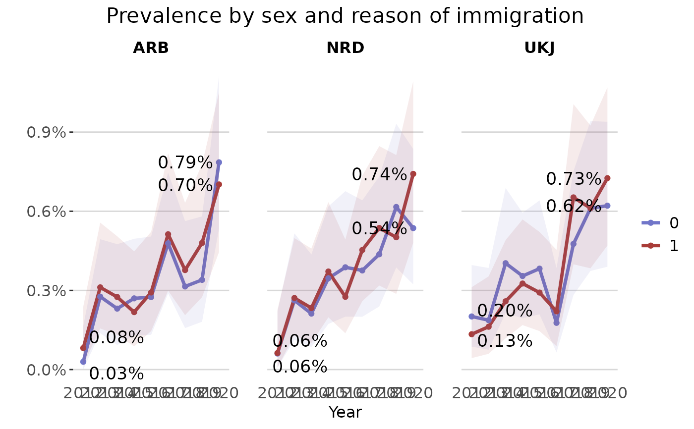
plot_rates(prev_series,
date_col = "year",
rate_col = "prev_rate",
plot_type = "line",
grouping_var = "sex",
facet_var = "innvandringsgrunn",
palette = "fhi_colors",
CI_lower = "ci_results_lower",
CI_upper = "ci_results_upper",
plot_title = "Prevalence by sex and reason of immigration",
x_name = "Year",
start_end_points = TRUE)